Gradient descent, visually explained
Cost function is a surface. Derivative is slope. θ = θ − α·∇J(θ). Every neural net you've ever heard of is this rule, repeated.
Gradient descent, visually explained
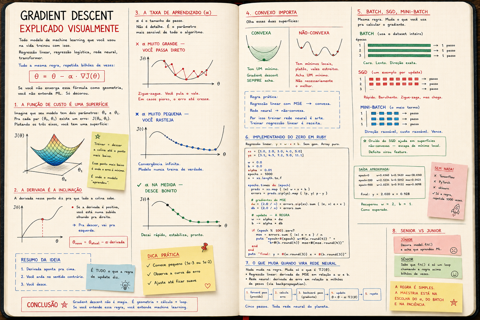
Every machine learning model you've ever used was trained with this.
Linear regression, logistic regression, neural net, transformer.
All the same rule, repeated billions of times:
θ = θ - α · ∇J(θ)
If you don't see this formula as geometry, you don't understand ML. You memorized it.
The cost function is a surface
Imagine your model has two parameters: θ₀ and θ₁.
For each pair (θ₀, θ₁) there's an error: J(θ₀, θ₁).
Plot the three axes and you get a surface:
        J(θ)
         │
         │       ╱╲
         │      ╱  ╲___
         │     ╱       ╲___
         │    ╱             ╲___
         │___╱                  ╲___
         └─────────────────────────── θ
Training = walk down the hill until you reach the lowest point.
That lowest point is where the error is minimum. It's where the model "learned".
No mystery. It's geometry.
The derivative is the slope
Pick any point on the surface.
The derivative at that point tells you which way the hill goes up.
J(θ)
 │
 │    •  ← you are here
 │   ╱
 │  ╱   derivative > 0  → goes up to the right
 │ ╱                    → so go left to descend
 │╱
 └────────────────── θ
If the derivative is positive, you're on a slope facing right.
To go down, go left. That is: subtract from your current position.
That's all the update rule says:
θ_new = θ_current - α · derivative
Derivative points up. You walk the opposite way. You descend.
The learning rate (α)
α is the step size.
Not a detail. It's the most sensitive parameter in the entire algorithm.
α too large — you overshoot
J(θ)
 │  •
 │ ╱ ╲       •
 │╱   ╲     ╱
 │     ╲   ╱   •
 │      ╲ ╱   ╱
 │       •───╱
 └──────────────── θ
Zigzag. You skip the valley. In worse cases, the error even grows.
α too small — you crawl
J(θ)
 │•
 │ •
 │  •
 │   •
 │    •
 │     •     (1000 epochs later, still in the same place)
 └──────────────── θ
Infinite convergence. Model never really trains.
α just right — clean descent
J(θ)
 │•
 │  •
 │     •
 │        •
 │           •
 │              •──•──•
 └──────────────────────── θ
Drops fast, settles, done.
Finding that α is half the job in practice.
Convex matters
Look at these two surfaces:
Convex                       Non-convex

   ╲           ╱             ╲    ╱╲   ╱
    ╲         ╱               ╲  ╱  ╲ ╱
     ╲       ╱                 ╲╱    •
      ╲     ╱                   •
       ╲   ╱                  (local minimum)
        ╲ ╱
         •
   (global minimum)
Linear regression with MSE → convex. One minimum. Gradient descent always finds it.
Neural net → non-convex. Local minima, plateaus, narrow valleys. Gradient descent finds a minimum. Not necessarily the best one.
That's why training a neural net is art. And training linear regression is a recipe.
Batch, SGD, mini-batch
Same rule. Changes what you use to compute the gradient.
Batch — the whole dataset per update
epochs
 1   ████████████████  → compute ∇J → 1 step
 2   ████████████████  → compute ∇J → 1 step
 3   ████████████████  → compute ∇J → 1 step
Expensive. Slow. But the direction is exact.
SGD — one example per update
 1   █  → ∇ → step
 1   █  → ∇ → step
 1   █  → ∇ → step
 ...
Fast. Noisy. Zigzags, but gets there.
Mini-batch — the middle ground (what everyone uses)
 1   ████  → ∇ → step
 1   ████  → ∇ → step
 1   ████  → ∇ → step
Reasonable direction, reasonable cost. Wins.
SGD's noise even helps on non-convex surfaces — it escapes local minima.
Bug became feature.
Implementing it from scratch in Ruby
Linear regression. y = w·x + b. No gem. Plain arrays.
# data: y ≈ 2x + 1 with a bit of noise
xs = [1.0, 2.0, 3.0, 4.0, 5.0]
ys = [3.1, 4.9, 7.2, 9.0, 11.1]

w = 0.0
b = 0.0
alpha = 0.01
epochs = 1000
n = xs.length.to_f

epochs.times do |epoch|
  # forward: prediction
  preds = xs.map { |x| w * x + b }

  # errors
  errors = preds.zip(ys).map { |p, y| p - y }

  # MSE gradients
  #   ∂J/∂w = (2/n) Σ (pred - y) · x
  #   ∂J/∂b = (2/n) Σ (pred - y)
  dw = (2.0 / n) * errors.zip(xs).sum { |e, x| e * x }
  db = (2.0 / n) * errors.sum

  # update — THE RULE
  w -= alpha * dw
  b -= alpha * db

  if (epoch % 100).zero?
    mse = errors.sum { |e| e * e } / n
    puts "epoch=#{epoch} w=#{w.round(4)} b=#{b.round(4)} mse=#{mse.round(4)}"
  end
end

puts "final: y = #{w.round(3)} x + #{b.round(3)}"
Approximate output:
epoch=0   w=0.4140 b=0.1420 mse=58.4140
epoch=100 w=2.1234 b=0.5012 mse=0.0421
epoch=900 w=2.0231 b=0.9132 mse=0.0098
final: y = 2.020 x + 0.928
It recovered w ≈ 2, b ≈ 1. As expected.
No TensorFlow. No PyTorch. No sklearn.
Just the rule, repeated 1000 times.
What changes when it becomes a neural net
Nothing changes in the rule. What changes is what ∇J(θ) is.
- linear regression: derivative of MSE with respect to
wandb. Closed form. - neural net: derivative of the error with respect to millions of weights. Closed form too — but via backpropagation, which is the chain rule applied layer by layer.
The heart of the algorithm is always:
1. forward pass — compute prediction
2. compute error
3. backward pass — compute gradient
4. update — θ = θ - α · ∇J(θ)
5. repeat
Five steps. Every neural net on the planet.
Senior vs junior
- junior memorizes
model.fit()and thinks they learned ML - senior knows that
fit()is just a loop calling the rule above
When the model doesn't converge, the junior switches frameworks.
The senior looks at the learning rate. The batch size. The data scale. The weight initialization.
Because they know exactly what's happening on the descent.
Conclusion
Every neural net you've ever heard of — GPT, ResNet, AlphaGo — is the same formula:
θ = θ - α · ∇J(θ)
Repeated.
Billions of times.
Across billions of parameters.
With gradients computed via backprop.
Nothing else.
The rest is engineering: how to compute the gradient fast, how to avoid bad minima, how not to blow up memory.
But the core is a hill and someone walking down it, one step at a time.
If you understood that, you understood ML.