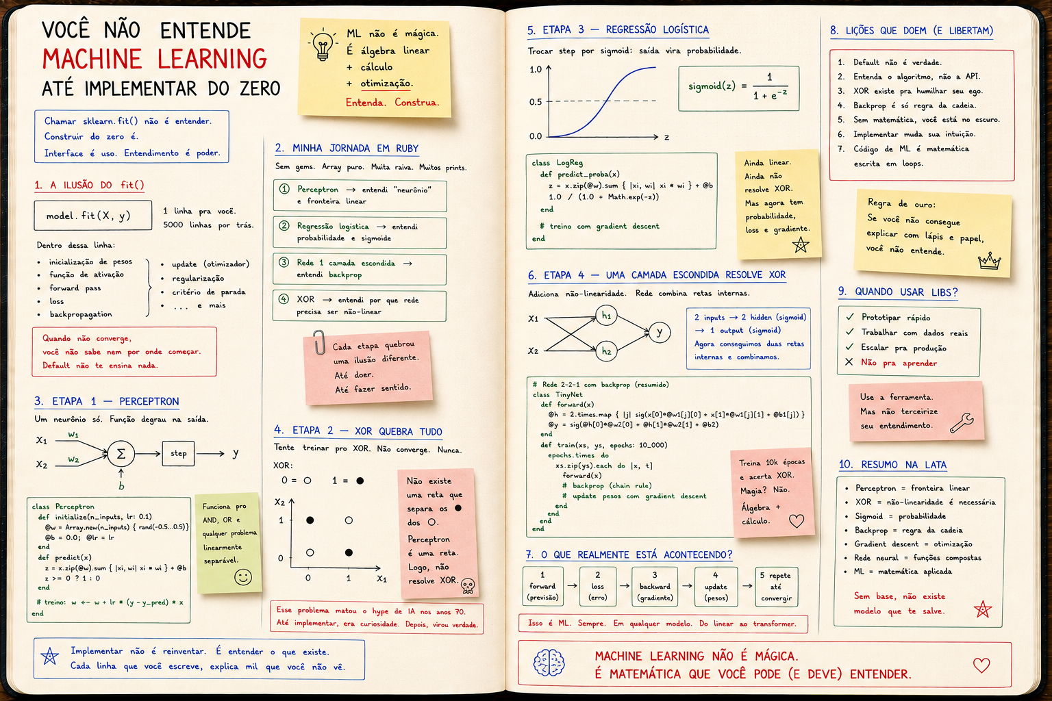
You don't understand Machine Learning until you implement it from scratch
Calling sklearn.fit() isn't understanding. Building a perceptron, logistic regression and a net that solves XOR in Ruby is. ML is algebra and optimization — not magic.
You don't understand Machine Learning until you implement it from scratch
There's a huge difference between:
from sklearn.linear_model import LogisticRegression
model = LogisticRegression().fit(X, y)
…and knowing what those two lines are doing.
The first is usage. The second is understanding.
And the whole industry confuses the two.
The fit() illusion
You imported. You called .fit(). The model trained. 92% accuracy.
Did you "do ML"?
No. You used the interface.
┌──────────────────────────────────────┐
│   model.fit(X, y)                    │
│                                      │
│   what you see: 1 line               │
│   what's inside: 5000 lines          │
└──────────────────────────────────────┘
Inside that line:
- weight initialization (with what strategy?)
- choice of activation function
- forward pass
- loss computation
- backpropagation
- weight update with some optimizer
- stopping criterion
- regularization
You chose none of that. The default chose for you.
Then comes the day the model doesn't converge. And you don't even know where to start.
My experience: an ML lib in Ruby
I decided to learn ML the way I learned everything in programming: by writing, not by reading.
I didn't care if it would be slow. I didn't want a gem. I wanted to see the algorithm bleed.
In Ruby. Plain arrays. No NMatrix, no Numo, nothing.
The path was this:
1. Perceptron           → got "neuron" and linear boundary
2. Logistic regression  → got probability and sigmoid
3. 1-hidden-layer net   → got backprop
4. XOR                  → got why a net needs non-linearity
Each step broke a different illusion.
Step 1 — Perceptron
A perceptron is a single neuron.
     x1 ──w1──┐
              ├──[ Σ ]──[ step ]── y
     x2 ──w2──┘
              ↑
              b
Weights w, bias b, weighted sum, step function on the output.
class Perceptron
  def initialize(n_inputs, lr: 0.1)
    @w = Array.new(n_inputs) { rand(-0.5..0.5) }
    @b = 0.0
    @lr = lr
  end

  def predict(x)
    z = x.zip(@w).sum { |xi, wi| xi * wi } + @b
    z >= 0 ? 1 : 0
  end

  def train(xs, ys, epochs: 20)
    epochs.times do
      xs.zip(ys).each do |x, y|
        pred = predict(x)
        error = y - pred
        @w = @w.zip(x).map { |wi, xi| wi + @lr * error * xi }
        @b += @lr * error
      end
    end
  end
end

# logical AND
xs = [[0,0],[0,1],[1,0],[1,1]]
ys = [0, 0, 0, 1]

p = Perceptron.new(2)
p.train(xs, ys)
xs.each { |x| puts "#{x.inspect} → #{p.predict(x)}" }
Works for AND. For OR. For any linearly separable problem.
Then came the slap.
Step 2 — XOR breaks everything
I tried training for XOR:
xs = [[0,0],[0,1],[1,0],[1,1]]
ys = [0, 1, 1, 0]
Doesn't converge. Ever.
And that's when I understood, for the first time, what linear separability means.
Plot XOR on a plane:
   x2
    │
  1 ●   ○      ● = class 1
    │           ○ = class 0
    │
  0 ○   ●
    │
    └────────── x1
        0   1
There's no straight line separating the ●s from the ○s. None.
A perceptron is a line. So a perceptron can't solve XOR.
This is the problem that killed the AI hype of the 70s.
And until I implemented it, it was just a textbook curiosity.
After implementing it, it became knowledge.
Step 3 — Logistic regression
Swapping step for sigmoid solves something important: the output becomes a probability.
sigmoid(z) = 1 / (1 + e^-z)

  1.0 │            ___________
      │         __/
  0.5 │      __/
      │   __/
  0.0 │__/
      └──────────────────────── z
And since sigmoid is differentiable, you can actually use gradient descent.
class LogReg
  def initialize(n_inputs, lr: 0.1)
    @w = Array.new(n_inputs, 0.0)
    @b = 0.0
    @lr = lr
  end

  def sigmoid(z) = 1.0 / (1.0 + Math.exp(-z))

  def predict_proba(x)
    z = x.zip(@w).sum { |xi, wi| xi * wi } + @b
    sigmoid(z)
  end

  def train(xs, ys, epochs: 1000)
    n = xs.length.to_f
    epochs.times do
      dw = Array.new(@w.length, 0.0)
      db = 0.0
      xs.zip(ys).each do |x, y|
        p = predict_proba(x)
        err = p - y
        @w.each_index { |i| dw[i] += err * x[i] }
        db += err
      end
      @w.each_index { |i| @w[i] -= @lr * dw[i] / n }
      @b -= @lr * db / n
    end
  end
end
Still linear. Still doesn't solve XOR. But now you have probability, gradient descent, and a differentiable loss.
One thing is missing: depth.
Step 4 — One hidden layer solves XOR
Add a layer of neurons in the middle:
   x1 ─┐    ┌──[ h1 ]──┐
       ├────┤          ├──[ y ]
   x2 ─┘    └──[ h2 ]──┘
Each h is a non-linear transformation of the input. The output combines the hs.
Now the net can draw two lines internally and combine them. XOR becomes separable.
class TinyNet
  # 2 inputs → 2 hidden (sigmoid) → 1 output (sigmoid)
  def initialize(lr: 0.5)
    @w1 = Array.new(2) { Array.new(2) { rand(-1.0..1.0) } } # 2x2
    @b1 = Array.new(2, 0.0)
    @w2 = Array.new(2) { rand(-1.0..1.0) }                  # 2
    @b2 = 0.0
    @lr = lr
  end

  def sig(z) = 1.0 / (1.0 + Math.exp(-z))
  def dsig(s) = s * (1 - s)

  def forward(x)
    @h = Array.new(2) do |j|
      sig(x[0] * @w1[j][0] + x[1] * @w1[j][1] + @b1[j])
    end
    @y = sig(@h[0] * @w2[0] + @h[1] * @w2[1] + @b2)
  end

  def train(xs, ys, epochs: 10_000)
    epochs.times do
      xs.zip(ys).each do |x, target|
        # forward
        out = forward(x)

        # backward (chain rule)
        d_out = (out - target) * dsig(out)
        d_h = Array.new(2) { |j| d_out * @w2[j] * dsig(@h[j]) }

        # updates
        2.times { |j| @w2[j] -= @lr * d_out * @h[j] }
        @b2 -= @lr * d_out

        2.times do |j|
          @w1[j][0] -= @lr * d_h[j] * x[0]
          @w1[j][1] -= @lr * d_h[j] * x[1]
          @b1[j]    -= @lr * d_h[j]
        end
      end
    end
  end
end

xs = [[0,0],[0,1],[1,0],[1,1]]
ys = [0, 1, 1, 0]

net = TinyNet.new
net.train(xs, ys)
xs.each { |x| puts "#{x.inspect} → #{net.forward(x).round(3)}" }
Expected output:
[0, 0] → 0.04
[0, 1] → 0.96
[1, 0] → 0.96
[1, 1] → 0.05
Solved XOR. In Ruby. In 60 lines. With no gem at all.
And only then did I understand backprop. Because I wrote the chain rule by hand.
What fit() hides
Look at everything that showed up in this exercise:
┌─ forward pass ─────────────────────────┐
│  composition of non-linear functions   │
└────────────────────────────────────────┘
┌─ loss ─────────────────────────────────┐
│  how the error is measured             │
└────────────────────────────────────────┘
┌─ backprop ─────────────────────────────┐
│  chain rule across layers              │
└────────────────────────────────────────┘
┌─ weight init ──────────────────────────┐
│  zero breaks. small random works       │
└────────────────────────────────────────┘
┌─ activation ───────────────────────────┐
│  step, sigmoid, tanh, ReLU…            │
│  each one changes what the net can do  │
└────────────────────────────────────────┘
┌─ learning rate ────────────────────────┐
│  big α explodes, small α stalls        │
└────────────────────────────────────────┘
All of that disappears behind one sklearn line.
You'll never understand ML staring at that line.
Senior vs junior
- junior imports a model, tunes hyperparameters until accuracy goes up, and moves to the next task
- senior knows, for each line of
fit(), which operation is happening and why
The junior treats the model as a black box.
The senior treats it as algebra with a loop.
Salary difference. And difference in the kind of problem each can actually solve.
Why this changes everything
When you implement it:
- you understand why normalizing data matters (gradient explodes otherwise)
- you understand why initialization matters (zero makes every neuron learn the same thing)
- you understand why ReLU won (sigmoid saturates, gradient vanishes)
- you understand why depth helps (more composition = more expressive power)
- you understand why big nets need lots of data (more parameters = more degrees of freedom)
None of that lands by reading a blog post.
It lands by writing the code.
Conclusion
Machine Learning is not magic.
It's linear algebra, calculus, and optimization — orchestrated in a loop.
And you only see that when you write the loop with your own hands.
sklearn, PyTorch, TensorFlow are excellent tools — once you understand.
Before that, they're layers hiding what you needed to learn.
If you've never implemented a perceptron, a logistic regression, and a one-hidden-layer net, you don't know ML.
You know the API.
And APIs change. Fundamentals don't.